When Data Processing is thought about these days, computers are in the picture mostly.
So understanding how real time data can be interpreted and modified by discrete state machines becomes essential.
Yes, I’m going to talk about Discrete Signal Processing, with all necessary introductions. I’m also expecting you know high-school calculus, and what \(e^{j\theta} = cos(\theta) + j sin(\theta)\) means.
Apart from this, to ensure you’re on the same page, let’s discuss over frequencies, and why consider them at all.
Need for defining Frequency
When I was first introduced to \(f = \frac{1}{t}\) during a lecture on Simple Harmonic Motion, where \(f\) is in \(Hz\) if \(t\) is in \(sec\). I ignored this topic. It seemed too trivial for being worthwhile. Why need to discuss about such a term at all, if time \(t\) is already sufficient to describe signals.
It turns out, as a general rule of thumb, the scientific community runs because there exists multiple perspective of the same thing. It’s easier to understand the motion of a pendulum in terms of energy than the laws of force. It’s also easier to understand materials in terms of chemical composition instead of molecular interactions.
True, level of abstraction differs in each perspective, but what’s special in the case of \(f\) v/s \(t\) is that they are not just different, but are representing exactly the same thing, no details missed whatsover.
Abstraction is the process of taking away or removing characteristics from something to reduce it to some set of essential characteristics. Making things simpler, and more general.
Despite of being equivalent, one perspective might be much more insightful than the other, depending on the case of course.
The bigger picture to keep in mind is, what representation makes you understand the phenomenon at hand from axioms (or principles you agree that are fundamental), and what helps you predict other useful information about the same.
From information, you can only derieve other information. Usecase is a matter of different concern, which also I’ll touch upon.
So here we have it, \(f\) might be significant.
Different Domain
After a few years, I stumbled upon the term of fourier analysis, and heard how it can solve many problems which are extremely difficult to deal with. Unsurprisingly, I searched it up, saw a video, and thought wow, downright hits as a usual 3b1b video does!
But what to do with it now? So it swept out of my mind, until our curriculum induced it into a course.
First axiom
You know that sinusoids, \(sin(x)\) and \(cos(x)\) together, are periodic functions.
It turns out, shown by Joseph Fourier in 1800s, that any periodic signal can be said to be a weighted sum of different kinds of sinusoids.
Take it for granted now. I won’t prove it.
Let’s understand the statement again. If you saw it as “Periodic signal - combination of sinusoids”, observe again, there are a few vague terms in there.
Sinusoids and frequencies
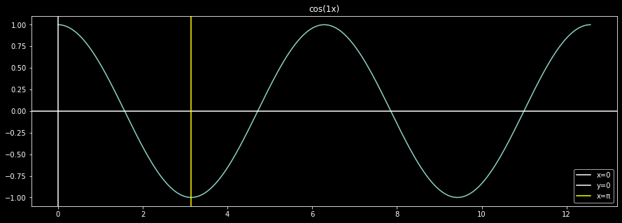
Think about \(cos(x)\). It’s plot is something like:
Consider now \(cos(2x)\). Something like:
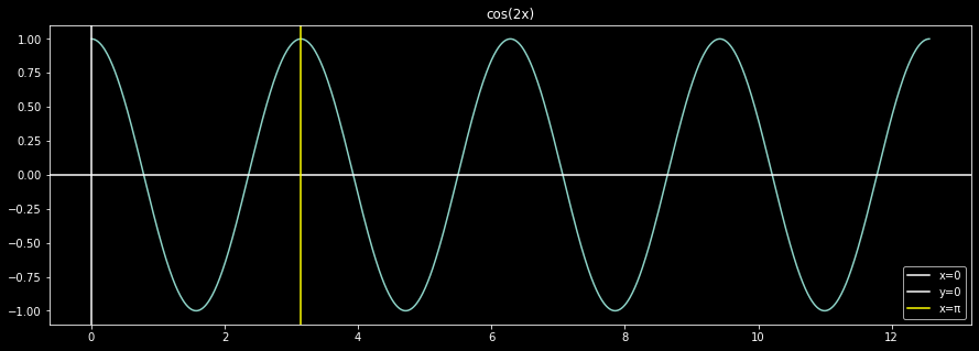
Something changed. The function shrunk along the x-axis. Another way to say it, the function changes faster in the second case. More specifically, before the period of the function was \(2\pi\), which now decreased to \(\pi\). Rename the x-axis as the time axis (another beauty of abstraction). It’s time period decreased. Now from the above definition, it’s frequency increased, from \(\frac{1}{2\pi} = 0.15915 \,\mathrm{Hz}\) to \(\frac{1}{\pi} = 0.31831 \,\mathrm{Hz}\).
Admittedly, working with such frequencies seems cumbersome, so for sinusoids, we opt for angular frequencies, defined as \(2\pi f\), denoted as \(\omega\).
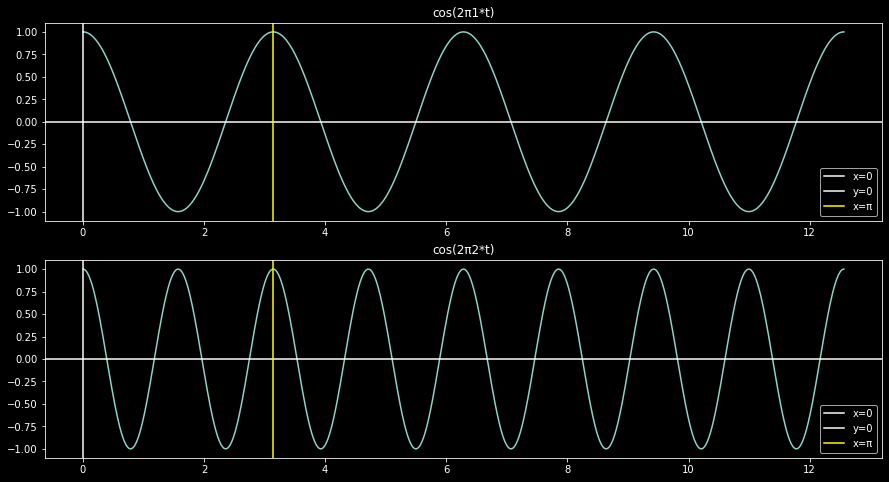
Now the frequencies involved are much nicer, \(1\) and \(2\) respectively. Doing so translated to change in period from \(2\pi\) to \(1\).
Weighted combination of different sinusoids
Different sinusoids means sinusoids of different frequencies. And not just any set of frequencies.
Let the \(x(t)\) periodic signal under consideration have a period of \(T\). So it’s angular frequency is \(\omega_0 = \frac{2\pi}{T}\).
Claim of Joseph Fourier was, the periodic signal can be decomposed to/is weighted sum of sinusoids with frequencies as integral multiples of \(\omega_0\).
\(x(t) = w^s_0 sin(0\:\omega_0 t) + w^s_1 sin(1\:\omega_0 t) + w^s_2 sin(2\:\omega_0 t) + \cdots\)
\(\;\;\;\;\;\;\;\;\;\;\;\;\; + w^c_0 cos(0\:\omega_0 t) + w^c_1 cos(1\:\omega_0 t) + w^c_2 cos(2\:\omega_0 t) + \cdots\)
Yes, all positive integral multiples.
Represented more neatly as:
\[\begin{aligned}
x(t) & = \sum_{n=0}^{\infty} a_n cos(n\omega_0 t) + \sum_{n=0}^{\infty} b_n sin(n\omega_0 t) \\
& = \sum_{n=0}^{\infty} a_n cos(n\omega_0 t) + b_n sin(n\omega_0 t)
\end{aligned}\]
Here, complex exponentials are included to simplify the representation.
\[a_n cos(n\omega_0 t) + b_n sin(n\omega_0 t) = \frac{a_n + b_n}{2} e^{j n\omega_0 t} + \frac{a_n - b_n}{2} e^{-j n\omega_0 t} \\
\begin{aligned}
x(t) & = \sum_{n=0}^{\infty} \frac{a_n + b_n}{2} e^{j n\omega_0 t} + \frac{a_n - b_n}{2} e^{-j n\omega_0 t} \\
\end{aligned}\]
\[\tag{1} x(t) = \sum_{n=-\infty}^{\infty} c_n e^{j n\omega_0 t}\]
Good enough, so if you know \(c_n\)’s for a signal, you can combine them as above.
But what about computing \(c_n\) in the first place, if your signal \(f(t)\) is given?
We use orthogonality.
Orthogonality
Two functions are defined to be orthogonal for \(t \in (a, b)\) if
\[\langle u, v\rangle = 0 \iff \int_{a}^{b} u(t) v^*(t) dt = 0\]
It’s good to know that the complex exponential family are orthogonal w.r.t. each other.
\[\langle e^{j \omega nt}, e^{j \omega mt}\rangle =
\begin{cases}
0 & n\neq m \\
1 & n = m \\
\end{cases} \\
\ni t \in (a, a + 2\pi) \;\; \forall a \in \mathbb{Z}\]
Proof as follows
\[\begin{aligned}
\int_{a}^{a + 2\pi} e^{j \omega mt} \cdot e^{-j \omega nt} dt & = \int_{a}^{a + 2\pi} e^{j \omega (m-n)t} dt \\
& = \frac{e^{j \omega (m-n)t}}{j \omega (m-n)} \Biggr|_{a}^{a + 2\pi} \\
& = \frac{e^{j \omega (m-n) (a + 2\pi)} - e^{j \omega (m-n) (a)}}{j \omega (m-n)} \\
& = e^{j \omega (m-n) (a)}\frac{e^{j 2\pi\omega (m-n)} - 1}{j \omega (m-n)} \\
& = \begin{cases}
0 & n\neq m \\
1 & n = m \\
\end{cases} \\
\end{aligned}\]
Using this concept in Eqn (1), consider the following expression
\[\begin{aligned}
\int_{0}^{2\pi} x(t) e^{-j\omega_0 nt} dt & = \int_{0}^{2\pi} \underbrace{\Big(\sum_{m=-\infty}^{\infty} c_m e^{j m\omega_0 t}\:\Big) e^{-j\omega_0 nt}}*{c_n} dt \\
& = c_n \int*{0}^{2\pi} dt
\end{aligned}\]
\[\tag{2} c_n = \frac{1}{2\pi} \int_{0}^{2\pi} x(t) e^{-j\omega_0 nt} dt\]
Lo behold, you have completed the Fourier Series Analysis that includes Eqn (1) and (2), which is the first step towards the idea of decomposing data into, well, simpler data.
Sinusoids are simple to understand, they come up many places in academia or reality (most places via approximations, but still).
You won’t find the following function as common though:
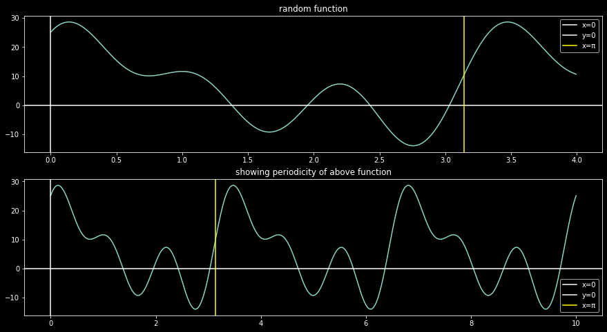
This can be decomposed to the following sinusoids, given \(\omega_0 = 0.6\pi \implies T = 3.333\)
\[\begin{aligned}
f(t) & = 5.535 cos(0\omega_0 t) + 8.379 cos(1\omega_0 t) + 2.417 cos(2\omega_0 t) + 8.804 cos(3\omega_0 t) \\
& + 4.204 sin(0\omega_0 t) + 8.809 sin(1\omega_0 t) + 6.841 sin(2\omega_0 t) + 1.414 sin(3\omega_0 t)
\end{aligned}\]
This was constructed as
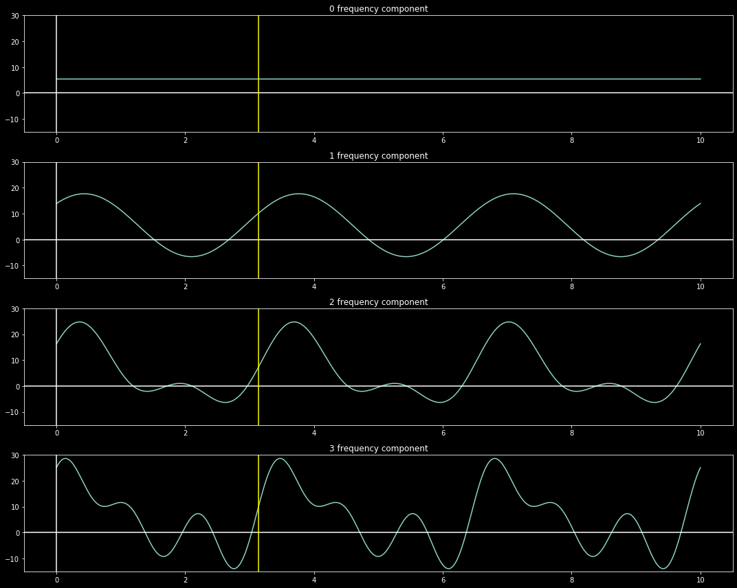
How is this useful now? Any periodic function, however large the period, can be decomposed as above. You can drop some higher order (larger frequency) terms, and the left function would still approximate the original one.
But you might say, usual data/signals are NOT periodic, also we would like to know how to deal with discrete signals, continuous signal processing is for analog peeps.
Nice points, so we will again leverage beauty of abstraction so move on to the next post.
dsp
basics
fourier-analysis