In Machine Learning models, our final optimization/goal usually ends in minimizing an objective function with respect to a set of model parameters, but what does that look like?
You know that
Our models are usually of the form \(f(X, \theta)\) where \(\theta\) is a set of parameters.
Optimizing a loss \(\mathcal{L}(\theta)\) encapsulates the constraint you want your model to learn as a single metric. If the loss itself is made from differentiable functions’ compositions, then using derivatives/gradients or backpropagation in general can yield the nudge you may want to give each of your weights to perform better on your dataset.
Loss hypersurface
\(\mathcal{L}(\theta)\) as you see it is actually \(\mathcal{L}(\theta, X, y)\), aka the loss value depends on the data in context. Whenever we are knudging the parameters \(\theta\), we are trying to optimize the value of that set of parameters such that the loss is minimised given \(X, y\).
Now comes the fun part, the Stochastic Batch Gradient Descent as you know, takes a set of samples from your dataset \((X_B, y_B)\), and calculates loss as well as the gradients on that particular batch! Note how it changes things. Your initial need was to optimize loss on your whole training dataset, but you’re optimizing it just over a batch. That’s what makes it different. The hypersurface of \(\mathcal{L}(\theta, X, y)\) v/s \(\theta\) is the key figure you need to keep in mind. There exists minima in its surface may and wouldn’t exactly coincide with the minima of \(\mathcal{L}(\theta, X_B, y_B)\). This is what leads to a different gradient than what it should be, inducing noise in your descent.
Also the graph of Loss v/s Parameters usage doesn’t end here. It’s a good perspective to keep in mind while working with your loss function. The graph yields an idea about weight initialisation method.
Better Weight Initialisation
Assume you want to obtain \(\theta\) that’s regularised and that optimizes the loss function. During initialisation usually what’s done is drawing of particular \(\theta_0\) that is then used for furthur optimization via descent or other means. Also descent requires you to calculate the loss value (forward-propagation) followed by weight update via gradient calculation per weight (back-propagation).
What I propose that it might be helpful to define a \(R^{D}\) dimensional “cube” and perform a grid search over any refinement of your liking.
Each grid vertex would correspond to a particular loss value. This would roughly give an idea of the location of optima prior to even starting any weight update. This works because your weights are anyways near zero, so such a cube would cover the range of your weights span.
There is one caveat of this method is that bias terms are usually not regularised because you can’t guarantee bias to be near zero. Ignoring that particular set of axes, you still would have a pretty good idea about the structure of Loss v/s Parameters space, which only comes out from forward propagation.
This is not costly because anyways forward propagation occurs thousands of times during training, so investing some initially to pick a better starting point leads to no harm.
Example of grid search initialisation
Imports needed
import numpy as np
from scipy.interpolate import griddata
import plotly
import plotly.graph_objs as go
Generate some dummy data
w_true = np.array([3.5, 7])
X = np.ones((45, 2))
X[:, 0] = np.random.random((45))*10
y = X @ w_true + (np.random.random((45)) + np.random.randn((45))) * 6
Take a batch for forward-propagation
# take a batch
y_b = y[:5]
X_b = X[:5]
Define your loss function, vectorize it (note that this doesn’t make it faster, but leads to automatic broadcasting)
@np.vectorize
def loss_(w1, w2):
    val = y_b - X_b @ np.array([w1, w2])
    return np.dot(val, val)
Perform Grid Search, you can always tweak these ranges
w1_grid = np.arange(-10, 10.1, 0.2)
w2_grid = np.arange(-50, 50.1, 0.2)
W1_grid, W2_grid = np.meshgrid(w1_grid, w2_grid)
Z = loss_(W1_grid, W2_grid)
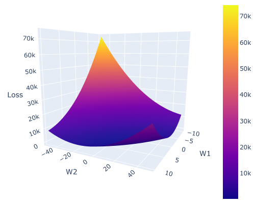
Now trying to check what value of W1 and W2 already leads to near minimum, one easy way might be
>> print(np.where(Z == np.min(Z)))
(array([295]), array([68]))
>> Z[295, 68], W1_grid[295, 68], W2_grid[295, 68]
(252.41028750748706, 3.5999999999999517, 9.000000000000838)
And these values are already pretty close to the real values of (3.5, 7)!
Note that we just used 5 data points out of the training set to estimate this.
This works out because all our data points are actually from the same original distribution, which is one of the fundamental assumptions we make when working with classical machine learning:
Training and Test (unseen) dataset are sampled from the same distributions
Plot the surface for visualization
plotly.offline.init_notebook_mode()
fig = go.Figure(go.Surface(x = W1_grid, y = W2_grid, z = Z))
fig.update_layout(
    height=400, width=500,
    margin=dict(l=0, r=0, t=0, b=0),
)
fig.update_scenes(xaxis_title_text='W1',
                  yaxis_title_text='W2',
                  zaxis_title_text='Loss')
fig.show()
Output Figure
I know people might argue that this seems infeasible to do for let’s say a neural network.
I would agree! Visualisation of that many dimensions is not easy or useful (or is it?), but you don’t need to visualize this, you can work with the weights corresponding to the minimum loss you obtained, or if you’ve multiple such minima, that’s great news, it means you can parallely work on all of them to find the global minima via descent.
Even though Deep Learning seems to be the norm these days, the classical Machine learning still works well and is essentially statistics. One of the rules for calculating gradients that keeps on being useful is
\[\frac{\partial (u^T A v)}{\partial x} = u^T A \frac{\partial v}{\partial x} + v^T A^T \frac{\partial u}{\partial x}\]
See ya.