Fourier Series from First Principles

2023-02-23 #signals #mathematics

The first time I met $f = \frac{1}{T}$ , in a lecture on simple harmonic motion, I ignored it. Time already seemed enough to describe a signal, so why introduce a second quantity that says the same thing?

Science often advances by having several perspectives on one thing. A pendulum is easier to understand through energy than through forces. What makes time and frequency special is that they are not two approximations of a signal. They are exact and complete descriptions of the same signal, with nothing lost in moving between them. One view can still be far more revealing than the other.

This post derives the first step of that idea, the Fourier series. I'll assume high-school calculus and familiarity with $e^{j\theta} = \cos\theta + j\sin\theta$ .

Frequency

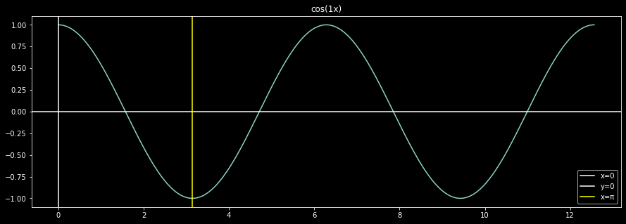
Here is $\cos(x)$ :

Plot of cos(x)

And here is $\cos(2x)$ :

Plot of cos(2x)

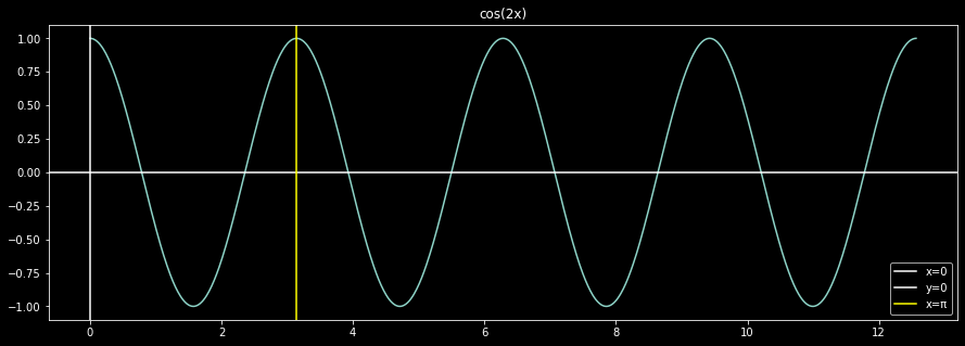
The second function changes faster. Its period drops from $2\pi$ to $\pi$ , so if we read the horizontal axis as time, its frequency rises from $\frac{1}{2\pi} \approx 0.159$ Hz to $\frac{1}{\pi} \approx 0.318$ Hz.

Those numbers are awkward, so for sinusoids we usually work with the angular frequency $\omega = 2\pi f$ . The same two signals now have $\omega = 1$ and $\omega = 2$ rad/s, and we can write any sinusoid simply as $\cos(\omega t)$ .

The claim

Joseph Fourier showed that periodic signals can be written as a weighted sum of sinusoids. Strictly, the signal has to be reasonably well behaved, but every signal you'd meet in practice is.

The sinusoids are not arbitrary. If $x(t)$ has period $T$ , define its fundamental frequency as $\omega_0 = \frac{2\pi}{T}$ . Then only integer multiples of $\omega_0$ are needed:

x(t) = a_0 + \sum_{n=1}^{\infty} \left( a_n \cos(n\omega_0 t) + b_n \sin(n\omega_0 t) \right)

This makes sense intuitively, since each of those sinusoids repeats every $T$ seconds, and so must any sum of them.

A neater form

Euler's formula lets us replace sines and cosines with complex exponentials:

\cos\theta = \frac{e^{j\theta} + e^{-j\theta}}{2}, \qquad \sin\theta = \frac{e^{j\theta} - e^{-j\theta}}{2j}

Substituting these in gives

a_n \cos(n\omega_0 t) + b_n \sin(n\omega_0 t) = \frac{a_n - jb_n}{2} e^{jn\omega_0 t} + \frac{a_n + jb_n}{2} e^{-jn\omega_0 t}

Collecting the terms into a single sum over positive and negative $n$ gives the compact form:

\tag{1} x(t) = \sum_{n=-\infty}^{\infty} c_n e^{jn\omega_0 t}

where $c_0 = a_0$ , and for $n > 0$ , $c_n = \frac{a_n - jb_n}{2}$ and $c_{-n} = \frac{a_n + jb_n}{2}$ .

If you know the $c_n$ , you can rebuild the signal. The remaining question is how to find them from $x(t)$ .

Orthogonality

Over an interval of one period, define the inner product of two functions as

\langle u, v \rangle = \int_{a}^{a+T} u(t)\, v^*(t)\, dt

Two functions are orthogonal when this is zero. The complex exponentials in equation (1) are orthogonal to one another. For $m \neq n$ ,

\begin{aligned} \int_{a}^{a+T} e^{jm\omega_0 t} e^{-jn\omega_0 t}\, dt &= \left. \frac{e^{j(m-n)\omega_0 t}}{j(m-n)\omega_0} \right|_{a}^{a+T} \\ &= e^{j(m-n)\omega_0 a}\, \frac{e^{j(m-n)2\pi} - 1}{j(m-n)\omega_0} \\ &= 0 \end{aligned}

The last step holds because $\omega_0 T = 2\pi$ and $e^{j2\pi k} = 1$ for every integer $k$ . When $m = n$ , the integrand is $1$ , so the integral is simply $T$ :

\langle e^{jm\omega_0 t}, e^{jn\omega_0 t} \rangle = \begin{cases} T & m = n \\ 0 & m \neq n \end{cases}

Extracting the coefficients

Multiply equation (1) by $e^{-jn\omega_0 t}$ and integrate over one period. Every term in the sum vanishes except the one with matching index:

\int_{0}^{T} x(t)\, e^{-jn\omega_0 t}\, dt = \sum_{m=-\infty}^{\infty} c_m \int_{0}^{T} e^{jm\omega_0 t} e^{-jn\omega_0 t}\, dt = c_n T

which gives us

\tag{2} c_n = \frac{1}{T} \int_{0}^{T} x(t)\, e^{-jn\omega_0 t}\, dt

Equations (1) and (2) are the whole of Fourier series analysis: one builds a signal from its coefficients, and the other recovers the coefficients from the signal.

An example

Sinusoids are simple. This function isn't:

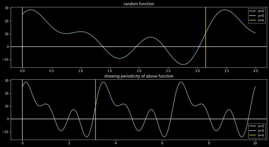
A periodic signal with an irregular shape

Yet with $\omega_0 = 0.6\pi$ , which means $T \approx 3.33$ , it is only a few sinusoids added together:

\begin{aligned} f(t) = 5.535 &+ 8.379\cos(\omega_0 t) + 2.417\cos(2\omega_0 t) \\ &+ 8.804\cos(3\omega_0 t) + 8.809\sin(\omega_0 t) \\ &+ 6.841\sin(2\omega_0 t) + 1.414\sin(3\omega_0 t) \end{aligned}

The figure below builds it up one harmonic at a time, starting from the constant term. Each panel adds the next frequency to the panels above it:

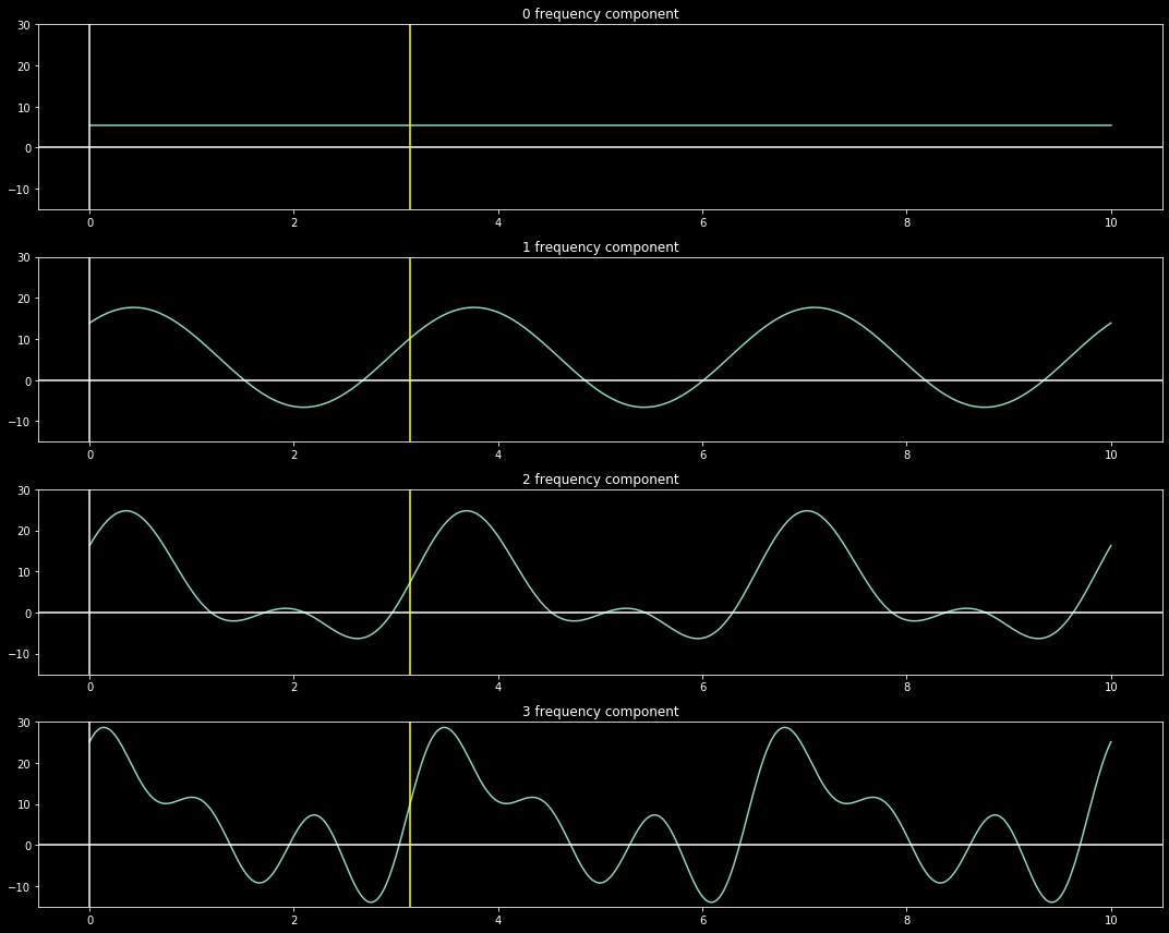
The signal built up cumulatively from its constant term and first three harmonics

This also shows why the decomposition is useful. Dropping the higher harmonics leaves a smoother approximation of the original signal, and the coefficients tell you how much each frequency matters.

Why this matters for control

Sinusoids have one more property that makes all of this worthwhile. Feed a complex exponential $e^{j\omega t}$ into a linear time-invariant system and the output is the same exponential, multiplied by a single complex number $H(j\omega)$ . That is the system's frequency response.

So once a signal is written as a sum of exponentials, the effect of a linear system on it reduces to scaling each term. Differential equations become multiplication, which is the foundation for Bode plots and much of classical control.

Real signals, of course, are rarely periodic, and computers only ever see samples of them. Handling those cases takes us to the Fourier transform and to discrete-time signal processing.

For a visual introduction to the same idea, I recommend 3Blue1Brown's video on the Fourier transform.